Chapter 1: Introducing Weights!

Welcome to the exciting world of machine learning!

In this chapter, we’ll start with the absolute basics – no technical background is needed.

Let’s get started!

We will start with a simple real-world example.

Let’s say you want to publish a post on Social Media, whether Facebook, Twitter (X), LinkedIn, or whatever…

Let’s say on Twitter (X)

image of a person thinking of his post on twitter if it will go viral or not

And before you push the post button, you want to predict if the post will go viral or not!

Of course, we are not going to use Black magic, Fortune Tellers, or Psychics here 😅.

We will try to do so by thinking about “conditions” or ‘factors” that make a post viral! That makes sense… ha!

For example, if a post is made on a weekend, it is likely to go viral. This is our prediction.

So we get an outcome:

Post on Weekend = viral ✅
Post on Weekday = Not viral ❌

This is a straightforward condition. If the condition (posting on the weekend) is met, the outcome is a viral post.

⚠️ Note that this is just a guess and has nothing to do with reality. We are just assuming that!

Somehow, a dummy prediction🤪!

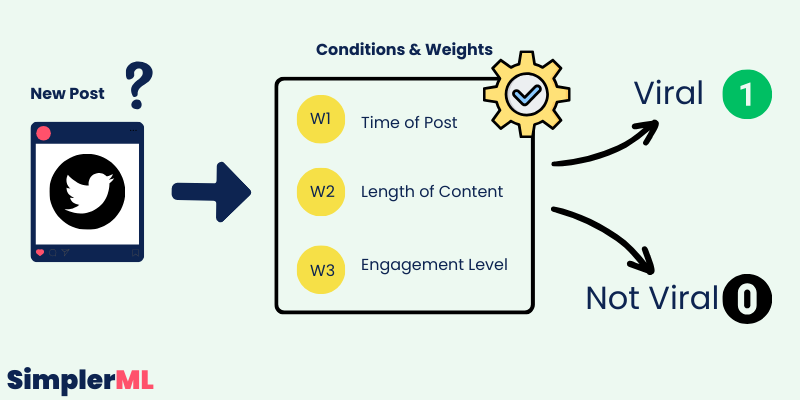
Let’s be a little smarter and use multiple conditions or factors, for example:

Condition 1: Time of the post (Morning, Afternoon, Evening).
Condition 2: Length of content (character count).
Condition 3: Day of the week (Weekday, Weekend).

Now, determining virality has become more complex since we want to check on multiple conditions to predict if the post will go viral or not. Yes?!

For example:

Posting a 200-character post in the evening on the weekend might be viral ✅
Posting 50 characters in the morning on a weekday might not be viral ❌

👉 With multiple conditions, the rules become more challenging to manage.

Introducing Weights 🤹‍♀️

What are weights?

If you think about it a little, each of the conditions we suggested may have contributed differently to making a post viral.

For example, the content length may have a 60% effect, while the Day of the week may have only 20%.

This is why we should think about giving weights for each condition!

We will Assign a numerical value to each condition based on its importance. (again, it is an assumption)

Time of Post: Weight = 0.3 (30%)
Length of Content: Weight = 0.5 (50%)
Day of the Week: Weight = 0.2 (20%)

Now, instead of just checking conditions, we calculate a score based on these weights.

💡Example :

A 200-character post posted in the evening on a weekday might get a score of:

0.5 (Length of Content) + 0.3 (Time of Post) + 0.1 (Day of the Week) = 0.9

Then, we compare this number to a threshold (a number that we assume makes a post viral, let’s say 0.8) – we will talk about this later.

In our case, 0.9 > 0.8, so the post is predicted to be viral.

This way, each condition contributes to the final decision, but with varying importance, reflected by their weights.

In Real Life, Weights are Hidden!

Going back to our example, we don’t know the weight for each condition. And this may even vary between platforms. Each platform sets its own weights based on its mission, algorithm, and how it works.

For instance, the publish time may be way more critical on Twitter than on YouTube.

Our primary goal is to find the proper weights so that when you give it an input, it can predict the output.

Here is a simple simulation of how weights affect our predictions:

Imagine you know the exact weights for each condition that makes a post viral. Then, you will not only predict virality but also have one billion followers in one week!

Ohh, I almost forgot that this book is about Machine learning😅 Let’s start then!

Machine learning is about finding and learning these weights, not only for social media posts. But for any use case where machine learning can help (more on that later)

How do we find the proper weights for each condition?

Let us stick to our example to keep things simple as before (I hope so)

What we will do now is look at posts already published, collect a list of both viral and non-viral posts, and record some data about the conditions we want to study and discover weights for. In our case, let’s collect the following data:

Time of Post (hour of the day)
Length of Content
Engagement Level

So we have like a table containing records for multiple posts, something like this:

Hour of Day (0-23)	Content-Length (chars)	Engagement Score (of 100)	Virality (0-1)
10	51	41.80	0
4	764	34.89	1
14	892	47.12	0

Perfect!

Now, with machine learning, we will figure out the patterns and relations between the inputs and outputs.

These are the weights! Another term for weights may be relations.

So, when we figure out the weights (relations), we can predict the output of new inputs.

In our case, new inputs are new posts.

Now that we’ve seen how assigning different weights to our conditions affects the outcome, we are beginning to touch on the essence of machine learning.

Let’s explore how this learning process works, stepping further into the world of machine learning, and how we can find the weights. Here is where the magic begins!

Finding weights with a random guess!

Since we are starting from scratch, we know nothing about the weights!

Our first basic dummy approach will be trying to guess them!

Let’s go back to your social media posts example.

We initially don’t know how important each factor (condition) is in determining a post’s virality. So, we assign random weights to each condition.

For simplicity, let’s say we assign weights on a scale from 0 to 1.

Here we are:

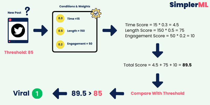
Time of Post: Weight = 0.3
Length of Content: Weight = 0.5
Engagement Level: Weight = 0.2

Example

Suppose we have a post with the following characteristics:

Posted at 15:00 (3 PM, represented as 15)
Content-Length: 150 characters
Engagement Level: 50 (average likes and comments)

We calculate the virality score as follows:

Time Score = 15 * 0.3 = 4.5
Length Score = 150 * 0.5 = 75
Engagement Score = 50 * 0.2 = 10

Total virality Score = 4.5 + 75 + 10 = 89.5

💡Setting a Threshold to test with.

Let’s set a threshold, say 85, to decide if a post is likely to be viral.

In our example, the score of 89.5 is above 85, so we predict this post will be viral.

Let’s review the weight Discovery process:

Initially, we assigned random weights to our conditions.

Each set of weights gives us some predictions about post-virality.

We then check how accurate these predictions are, like trying the guessed combination on a post that doesn’t belong to our dataset, but we know if it is viral or not, so this way, we can test our weights!

When we find a set of weights that gives us good predictions (meaning our predictions match the actual outcomes well), we’ve found a combination of weights that seems to work!

It is like Guessing the Numbers for a lock!

Imagine you’re trying to unlock a combination lock, but you don’t know the correct numbers. You try different combinations randomly. Suddenly, one combination clicks and the lock opens.

In machine learning, discovering a set of weights that accurately predicts outcomes (like whether a social media post will be viral) is similar to finding the right combination for a lock.

The moment we find a good combination of weights is very important. Here is why:

Validation of Our Approach: Discovering effective weights validates that our approach and understanding of the problem are on the right track.
Baseline for Improvement: This set of weights becomes a baseline. We know these weights work to some extent, so now we can try to improve them further. We are not blind anymore! We can optimize based on something from now on.

Diving Deeper – Real Application 🧐

Let’s go over the process of discovering weights step by step and in more detail to ensure you grasp the idea well before leveling up.

Step 0: Set the Goal

➡️ Predict If a Post will go viral on Twitter (X) based on multiple factors (conditions)

Step 1: Collect Data

We will collect some data on already published posts. We want both viral posts and non-viral.

We will have something like this:

Hour of Day	Content-Length	Engagement Score	Actual Virality
10	51	41.80	0
4	764	34.89	1
14	892	47.12	0
16	575	38.52	1
22	196	5.94	1

Hour of Day: This will be an integer ranging from 0 to 23, representing the 24 hours in a day.
Content-Length: This can be an integer representing the number of characters in the post. Let’s consider a range from 50 to 1000 characters.
Engagement Score: This could be a decimal number representing likes, shares, comments, etc., on a scale of 0 to 100.
Virality: if a post is viral, it is 1; if not, it is 0.

How did we collect this data?

Great question! The way we collect data for a project like this is very important and can be done in several ways. We will dive deeper into the details of data collection methods later in this book. But to give you a quick overview:

Manual Collection: In our scenario, This involves directly observing and recording data from social media posts. It’s time-intensive but can be very accurate for specific needs.
Using APIs: Social media platforms often provide Application Programming Interfaces (APIs), which are tools that allow us to automate the collection of large amounts of data.
Web Scraping: This method uses software and scripts to extract data from websites and social media platforms automatically. It’s useful for collecting data that isn’t readily accessible via APIs.
Public Datasets: Utilizing datasets released by government agencies, research institutions, or organizations, which can include social media data or related information.

Each method has its unique strengths and limitations. The choice of method depends on the project’s specific needs, the resources available, and the type of data required for the analysis. Don’t bother your head about how we got the data now. Let’s focus on our project.

We just collected it in some way 🕵️

Step 2: Adjusting Numbers – Normalization

Let’s zoom in and look again at our data. I picked two records:

Hour of Day	Content-Length	Engagement Score	Actual Virality
10	51	41.80	0
4	764	34.89	1

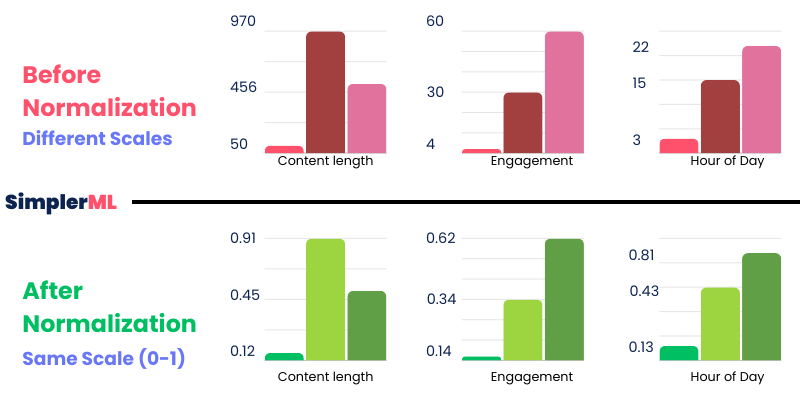
The hour of the day ranges from 0 to 23, while content length can range from 50 to 1000 or more. The Engagement Score can also range from 0 to 100.

So, we noticed that we have very different scales for each condition.

These different ranges and scales can directly affect the weight calculation process simply because** the machine learning program might incorrectly assume that the condition with a larger range (like the content length) is more important! **

Here comes the idea of Normalization, or adjusting the numbers into a similar scale or range.

Think of it like converting different currencies into one common currency to compare their values easily. Just as you would convert dollars and euros into a single currency to compare their values, normalization converts all features into a common scale.

How to Apply Normalization?

There are several methods to normalize data, but one common method is Min-Max normalization.

It rescales the values to a range of 0 to 1. Here is how:

Let’s say we are normalizing the “Content-Length” of a post.

Let’s take the second post in our dataset as an example.

Hour of Day	Content-Length	Engagement Score	Actual Virality
4	764	34.89	1

The original content length for this post was 764 characters.

Now, we find the Minimum (Min) and Maximum (Max) Values for content length in the Dataset:

In our case:

Minimum = 51

Maximum = 892

If you go back to the table, you will see that I colored it red and blue.

Ok, now we can calculate the normalized value of Content-Length using the min-max method as follows:

(Original Value – Minimum) / (Maximum – Minimum)

If you prefer Mathematical Formulas, here we are:

$\text{NormalizedValue} = \frac{\text{CurrentValue} - \text{MinimumValue}}{\text{MaximumValue} - \text{MinimumValue}}$

Whatever you prefer, let’s just apply this 3rd-grader formula to our numbers:

764 − 51 / 892 − 51 = 0.848

So 0.848 is the normalized ( scaled ) value of 764.

If we repeat the operation on all values in our data. Our dataset is transformed as follows:

Hour of Day	Content-Length	Engagement Score	Actual Virality
0.33	0.00	0.87	0
0.00	0.85	0.70	1
0.56	1.00	1.00	0
0.67	0.62	0.79	1
1.00	0.17	0.00	1

In this normalized dataset:

The “Hour of Day” values range from 0 (representing the earliest hour in our dataset) to 1 (the latest hour).
The “Content-Length” values are scaled between 0 (shortest content) and 1 (longest content).
The “Engagement Score” is also adjusted to a 0 to 1 scale, with 0 being the lowest engagement and one the highest.

Note that we will discuss data processing and normalization in more detail later in the book and with many more examples, but I tried here to introduce the concept with this simple example.

Let’s continue!

Step 3: Initialize a random set of weights.

As we mentioned before, we will try to guess the weights! So, we will assume a set of weights between 0 and 1!

Let’s say:

0.71 for Hour of Day
0.82 for Content-Length
0.11 for Engagement Score

Great! We have some weights we can test with.

Step 4: Predicting Popularity

Now that we have our normalized data and initial random weights, it’s time to see how well these weights predict a post’s popularity.

To illustrate this, consider the prediction as a straightforward calculation.

Each characteristic of a post (like the hour of the day, content length, and engagement score) is multiplied by its corresponding weight, which we had assumed randomly earlier.

The results of these multiplications are then summed up to yield a prediction score for each post.

For example, let’s take the second post in our dataset and apply our weights to its characteristics:

Hour of Day	Content-Length	Engagement Score	Actual Virality
0.00	0.85	0.70	1

Hour of Day Weight (0.71) × Hour of Day Score (0.00) + Content Length Weight (0.82) × Content Length Score (0.85) + Engagement Score Weight (0.11) × Engagement Score (0.70)

0.71 X 0.00 + 0.82 X 0.85 + 0.11 X 0.70 = 0.774

This score, 0.774 in our example, is our predicted popularity score for this particular post.

Now, we repeat the same process on all posts. We get something like this:

First Record: Popularity Score = 0.33
Second Record: Popularity Score ≈ 0.774
Third Record: Popularity Score ≈ 1.328
Fourth Record: Popularity Score ≈ 1.071
Fifth Record: Popularity Score ≈ 0.849

Perfect! We now have a list containing all the predicted popularity scores for each post.

Step 5: Measuring the Accuracy of Our Predictions

After predicting the popularity score for all posts, the next crucial step is to check how accurate this prediction is.

To do this, we compare our prediction scores with a pre-set threshold that defines what we consider as ‘viral.’

Let’s set a simple rule for our predictions:

If a post’s predicted score is higher than 0.85, we will classify it as viral.

This threshold is a value we decide on based on our understanding of what constitutes a viral post.

In our example, the predicted score for the second post is 0.774. Since this score is lower than our threshold of 0.85, we predict that this post will not go viral.

But! If we look into our dataset, we see that this post is actually Viral! So, we conclude that our prediction is wrong, which means our weights are wrong!

🔴We have an error.

Calculate Post Prediction Error

To calculate this error for each post prediction, we go through the following steps:

1- Classify each prediction as 0 or 1 based on the predicted score and threshold

We classify each post as viral (1) or not viral (0) by comparing its predicted score to the predefined threshold (0.85)

If the score is equal to or higher than the threshold, the post is classified as viral (predicted virality = 1).
If the score is lower than the threshold, the post is classified as not viral (predicted virality = 0).

2- Calculating The Error

In our dataset, we compare each post’s predicted virality (1 or 0) to its actual virality status (also 1 or 0).

The error for each post is the absolute difference between these two values:

If the predicted virality matches the actual status (both 1 or both 0), the error is 0 (no error).
If the predicted virality does not match the actual status (one is 1, and the other is 0), the error is 1 (misclassification).

Example 1: back to the second post:

Hour of Day	Content-Length	Engagement Score	Actual Virality
0.00	0.85	0.70	1

Predicted Score = 0.774 (less than 0.85) → Predicted Virality = 0
Actual Virality Value = 1
Error = 1 (misclassification: 1-0 )

Example 2: Let’s Check Post number 4 in the table:

Hour of Day	Content-Length	Engagement Score	Actual Virality
0.67	0.62	0.79	1

Predicted Score = 1.071 (greater than 0.85) → Predicted Virality = 1
Actual Virality Value = 1
Error = 0 (correct classification 1-1)

So, we get the errors for all posts in our dataset.

3- Average Error Calculation:

Now, let’s calculate the average error:

Average Error = Sum of All Errors / total number of posts

In our case:

0+1+1+0+0 / 5 = 2/5 = 0.4

So, the Average Error in our dataset for the assumed Weights is 0.4

Step 6: Calculating the Total Prediction Error

Okay, now we have the average error for our assumed weights, but the journey doesn’t end here. It is time to evaluate our guess (our assumed weights): Are they good or bad?

This is where the concept of an Error Threshold comes into play. Think of this threshold as a benchmark for performance. The closer we are to this number, the better our guess is.

In our case, we will set the error threshold to 0.2

So, we will compare the Calculated Average Error (0.4) from step 5 with our predefined Error Threshold (0.2).

If the average error is less than or equal to the Error Threshold, it means our model’s predictions are somehow accurate, and the weights are acceptable.

If the average error is greater than the Error Threshold, it indicates that our model’s predictions are NOT accurate enough, and we need to adjust the weights.

In our example, it is 0.4 > 0.2

It means our our guess failed. Hence, we cannot accept these weights!

Step 7: Repeat with a new guess!

Now what?

Simply start with a new guess and go again from step 3 to step 6 till we find a set of weights that works.

At that moment, we can congratulate ourselves on finding our lock’s secret key combination!

To be more accurate, we found a set of acceptable weights that can help us achieve our main goal.

What was the main goal?! ➡️ Predict If a Post will go viral on Twitter (X)

[Add an infographic showing all the steps again]

Iterative Improvement

Finding a good set of weights isn’t the end—it’s just the beginning. Machine learning’s real power comes from its ability to keep adjusting and improving these weights. This process is called iterative improvement, where we continuously refine and adjust our weights to make better predictions.

This method of using random weights and then adjusting them based on actual outcomes is a foundational concept in machine learning. It allows the Machine Learning Model to ‘learn’ from data and improve over time.

The Threshold

Remember I told you we’re gonna talk about the threshold?

So, let’s do it now!

Let’s Understand Threshold Using an Everyday Analogy:

The Amusement Park Ride

Imagine you’re at an amusement park, and there’s a roller coaster ride. However, to ensure safety, you must be at least 48 inches tall to ride.

1. Why the Height Requirement? (Objective)

Just like the roller coaster has a height requirement for safety, in our social media example, we set a threshold to decide if a post will be viral. It’s a kind of “safety check” to ensure our prediction (whether a post is viral or not) meets a certain standard.

2. How Tall Are Most People? (Data Distribution)

If most visitors are taller than 48 inches, many will get to ride. If many are shorter, fewer will. Similarly, in our example, we look at our data (posts) and see how many would be considered viral. This helps us decide where to set the threshold.

3. Avoiding Disappointment (Performance Metrics)

The park doesn’t want to disappoint too many kids or compromise safety. We also don’t want to label too many posts as viral when they’re not or miss out on ones that are truly viral.

4. Special Days (External Factors)

On a ‘kids day’, the park might lower the requirement slightly to let more kids enjoy. In social media, if there’s a special event or trend, we might adjust our threshold to reflect that.

Hope this journey helped you understand how you can set a threshold!

Okay, we are back now after a scary roller coaster ride. Let’s level up with more complex scenarios!

Hello Coders!

I understand that you may not be a coder, but if you’re curious about how the weight-guessing process works behind the scenes, this is a bonus peek “behind the scenes.”

Python Script on Gussing Weights

Here’s a Python script that you can play with. It demonstrates how to guess the weights so we can predict the virality of a Twitter post.

import random

import matplotlib.pyplot as plt

# Function to normalize data using max-min normalization

def normalize_data(data):

    norm_data = []

    for i in range(len(data[0])):

        col = [row[i] for row in data]

        min_val = min(col)

        max_val = max(col)

        norm_col = [(x - min_val) / (max_val - min_val) for x in col]

        norm_data.append(norm_col)

    return [list(x) for x in zip(*norm_data)]

# Twitter post data: Hour of Day, Content Length, Engagement Score

twitter_posts = [

    [10, 51, 41.80],

    [4, 764, 34.89],

    [14, 892, 47.12],

    [16, 575, 38.52],

    [22, 196, 5.94]

]

# Virality status (1 for viral, 0 for not viral)

ViralityStatus = [0, 1, 0, 1, 1]

# Normalize the Twitter post data

NormalizedPosts = normalize_data(twitter_posts)

# Function to initialize random weights for each feature

def initialize_weights(num_features):

    return [random.random() for _ in range(num_features)]

# Number of features in our data (3 in this case)

num_features = 3

# Randomly initializing the weights

RandomWeights = initialize_weights(num_features)

# Function to predict virality score

def predict_virality(post_features, weights):

    virality_score = 0

    for i in range(len(post_features)):

        virality_score += post_features[i] * weights[i]

    return virality_score

# Define a virality threshold

virality_threshold = 0.5

# Function to calculate the average error based on the threshold

def calculate_average_error(predictions, actuals):

    total_error = 0

    for i in range(len(predictions)):

        if predictions[i] >= virality_threshold:

            predicted_virality = 1

        else:

            predicted_virality = 0

        total_error += abs(predicted_virality - actuals[i])

    return total_error / len(actuals)

# Adjusting the threshold for average error

error_threshold = 0.2

# Storing the error for each iteration

errors = []

# Iterating to adjust weights

num_iterations = 1000

for i in range(num_iterations):

    PredictedVirality = []

    for features in NormalizedPosts:

        score = predict_virality(features, RandomWeights)

        PredictedVirality.append(score)

    AverageViralityError = calculate_average_error(PredictedVirality, ViralityStatus)

    errors.append(AverageViralityError)

    if AverageViralityError < error_threshold:

        print("Acceptable average error found!")

        break

    RandomWeights = initialize_weights(num_features)

# Plotting average error over iterations

plt.plot(errors)

plt.xlabel('Iteration')

plt.ylabel('Average Error')

plt.title('Average Error in Predicting Virality Over Iterations')

plt.show()

# Displaying final weights and lowest average error

print("Final Weights:", RandomWeights)

print("Lowest Average Error Achieved:", min(errors))

Let’s break it down:

Normalization: We start by normalizing the data to ensure all features are on a similar scale.
Random Weights: The script generates random initial weights for each feature (Hour of Day, Content-Length, Engagement Score).
Predicting Virality: It calculates a virality score for each post by multiplying features with weights and summing the results.
The Error Dance: The script iterates, constantly adjusting the weights and recalculating the average error compared to our ‘virality_threshold’. It stops when the error falls below an ‘error_threshold’.
Visualization: The included code even plots the average error over iterations, giving you a visual representation of the learning process.

Experiment Time!

Change the Thresholds: Play with the virality_threshold and error_threshold values. How does it affect the number of iterations and the final weights?
More Data, More Features: Expand the twitter_posts dataset. Can you add more features (e.g., number of hashtags, mentions)? How does this impact the results?

Important Note: This simplified example demonstrates the idea of weight guessing that we explained in this chapter. Real-world machine learning algorithms use more sophisticated methods for optimization.

For Non-Coders

Dont worry if you have not coded before. I have something for you, too.

Thousands of conditions!

Perfect. We’ve found a set of weights that work well with our few conditions. But what if our social media model had not just three factors but hundreds or maybe thousands?

Trying to guess the right combination of weights in this situation is like finding a needle in a haystack – actually, it’s more like finding a specific grain of sand on a beach!

The Challenge with a Huge Number of Conditions

Complexity Multiplies: With just a few conditions, it’s like juggling a few balls. But with thousands, it’s like juggling an entire circus worth of objects while blindfolded.

Guessing Becomes Impractical: If guessing the right combination for three conditions is like cracking a simple three-digit lock, then doing the same for thousands of conditions is like guessing the combination of a vault with a thousand dials. It’s not just difficult; it’s practically impossible!

Computational Burden: This isn’t just a mental challenge; it’s a computational one. The more conditions you have, the more possible combinations of weights there are, exponentially increasing the amount of time and resources needed to test each possibility.

Imagine trying to guess the WiFi password for a coffee shop that has a password composed of 100 random characters.

You sit down and start guessing: “coffee123”, “bestcoffeeintown”, “ilovecoffee”… As you add more characters, the likelihood of you hitting the correct password by random guesses becomes laughably impossible.

It’s the same with our weights – as we add more conditions, simply guessing becomes almost impossible.

Better Approach

Luckily, machine learning doesn’t rely on guesswork.

Instead, it uses awesome algorithms to find those ‘hidden’ weights and patterns all by itself.

In the next chapters, we’ll unravel how these algorithms work, one step at a time, breaking them down to ensure we understand exactly what’s going on.

And by the end, you’ll be able to use them to build super powerful machine learning models of your own!

I can’t wait to see what you create. See you in the next chapter!